Transformer Architecture
When I was new to AI and first encountered the Transformer Architecture, I felt overwhelmed by the sheer number of concepts and tutorials available to understand it. I noticed that some videos or articles assumed prior knowledge of natural language processing (NLP) concepts, while others were too lengthy and difficult to comprehend. To grasp the Transformer Architecture, I had to read numerous articles and watch several videos, and there were times when I got stuck due to a lack of basic knowledge that prevented me from fully understanding the topic, including:
With all the complexities involved, I have found it challenging to completely master this architecture. Therefore, I urge you to be patient and make sure to watch the video clips first, as the concepts are relatively easy to understand once explained. If we proceed step-by-step, starting from the basics and gradually moving towards more advanced topics, I am confident that you will soon be on the same page as me.
If you are new to LLM, be sure to check out my previous articles introducing the LLMs, which explains the basics of LLM and how it works.
High Level Overview
The Transformer model was first introduced in the paper 《Attention is all you need》 in 2017. The transformer architecture was intended for training language-translation purpose models. However, the team at OpenAI discovered that the transformer architecture was the crucial solution for character prediction. Once trained on the entirety of internet data, the model could potentially comprehend the context of any text and coherently complete any sentence, much like a human.
The model consists of two parts: the encoder and the decoder. In general, encoder-only architectures are proficient in extracting information from text for tasks like classification and regression, whereas decoder-only models specialize in generating text. For instance, GPT, which focuses on text generation, falls under the category of decoder-only models.
Let’s run through the key ideas of the architecture when training a model.
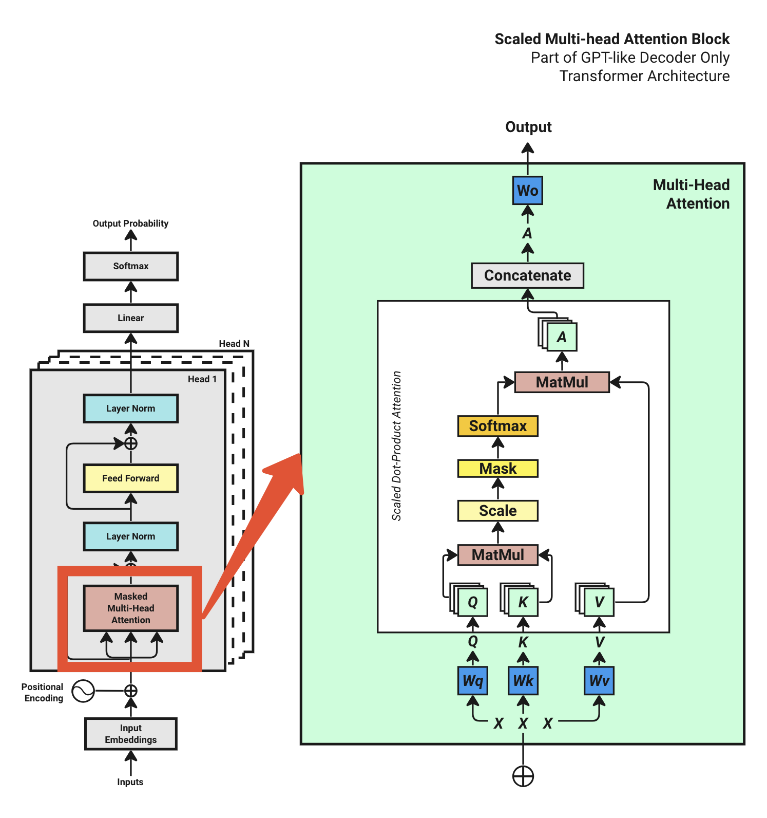
I drew a diagram to illustrate the training process of the GPT-like decoder-only transformer architecture:
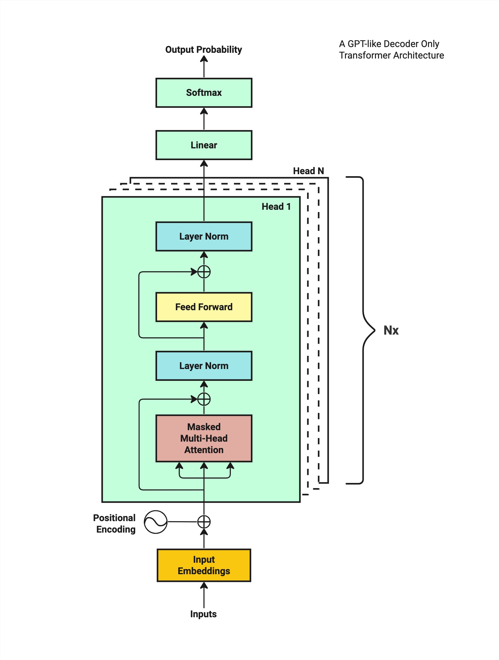
First, we require a sequence of input characters as training data. These inputs are converted into a vector embedding format.
Next, we add a positional encoding to the vector embeddings to capture each character's position within the sequence.
Subsequently, the model processes these input embeddings via a series of computational operations, ultimately generating a probability distribution over possible next characters for the given input text.
The model assesses the predicted outcome against the actual subsequent character from the training dataset, adjusting the probabilities or "weights" accordingly.
Finally, the model iteratively refines this process, updating its parameters continually to enhance the precision of future predictions.
Let's break into the details of each step.
Step 1 : Tokenization
Tokenization is the first step of a transformer model that:
Translates an input sentence into a format of number representations.
Tokenization is the process of dividing text into smaller units called tokens, which can be words, sub-words, phrases, or characters. Because breaking phrases into smaller pieces helps the model to identify the underlying structure of the text and process it more efficiently.
For example:
The above sentence can be cut into:
Chapter, , 1, :, , Building, , Rap, port, , and, , Capturing
which is tokenized as 10 numbers:
As you can see, number 220 is used to represent the white space character. There are many ways to tokenize charcters to integers. For our sample dataset, we will use tiktoken library.
For demonstration purpose, I'll use a small textbook dataset ( from Hugging Face) which contains 460k characters for our training.
File size: 450Kb
Vocab size: 3,771 (means unique words/sub-words)
Our training data contains a vocabulary size of 3,771 distinct characters. And the maximum number used to tokenize our textbook dataset is 100069, which is mapped to a character Clar.
Once we have the tokenized mapping, we can find the corresponding integer index for each character in the dataset. We will utilize these assigned integer indices as tokens moving forward, rather than using entire words when interfacing with the model.
Step 2 : Word Embeddings
To begin, let us construct a look-up table containing all the characters from our vocabulary. In essence, this table consists of a matrix filled with randomly initialized numbers.
Given the largest token number we have is 100069, and considering a dimension of 64 (with the original paper utilizing 512 dimensions, denoted as d_model), the resulting lookup table becomes a 100,069 × 64 matrix, this is called the Token Embedding Look-up Table. Represented as follows:
where each line represents a character (indexed by its token number) and each column represents a dimension.
For now, you can consider a 'dimension' as a characteristic or aspect of a character. In our case, we have designated 64 dimensions, which means we will be able to understand a character's textual meaning in 64 distinct ways, such as by categorizing it as a noun, verb, adjective, and so on.
Say, now we have an example training input of context_length of 16 which is:
" . By mastering the art of identifying underlying motivations and desires, we equip ourselves with "
Now, we retrieve the embedding vector for each tokenized character (or word) by using its integer index to look up the embedding table. As a result, we obtain their respective input embeddings:
[ 627, 1383, 88861, 279, 1989, 315, 25607, 16940, 65931, 323, 32097, 11, 584, 26458, 13520, 449]
In the transformer architecture, multiple input sequences are processed simultaneously in parallel, often referred to as multiple batches. Let's set our batch_size to be 4. Therefore, we will process four randomly selected sentences as our inputs at once.
each row represents a sentence; each column is the character from 0th to 15th position of that sentence.
In a result, we now have a matrix representing 4 batches of 16 characters inputs. The shape of this matrix is (batch_size, context_length) = [4, 16].
To recap, we defined an input embedding lookup table as a matrix of size 100,069 × 64 earlier. The next step is to take our input sequences matrix and map it onto this embedding matrix to obtain our Input Embedding.
Here, we will focus on breaking down each individual row of our input sequence matrix, starting with the first row. First, we reshape this opening row from its original dimensions of (1, context_length) = [1, 16] to a fresh format of (context_length, 1) = [16, 1]. Subsequently, we overlay this restructured row upon our previously established embedding matrix sized (vocab_size, d_model) = [100069, 64], thereby substituting the matching embedding vector for every single character present inside the given context window. The resulting output is a matrix with a shape of (context_length, d_model) = [16, 64].
First row of input sequence batch:
matrix shows one of the four rows after mapping
And we do the same to the rest of 3 rows, in the end we have 4 sets x [16 rows x 64 columns].
This results in the Input Embedding matrix with shape of (batch_size, context_length, d_model) = [4, 16, 64].
In essence, providing each word with a unique embedding allows the model to accommodate variations in language and manage words that have multiple meanings or forms.
Let us move forward with the understanding that our input embedding matrix serves as the expected input format for our model, even if we do not yet fully grasp the underlying mathematical principles at play.
Step 3 : Positional Encoding
In my opinion, positional encoding is the most challenging concept to grasp in the transformer architecture.
To summarize what positional encoding solves:
We want each word to carry some information about its position in the sentence.
We want the model to treat words that appear close to each other as “close” and words that are distant as “distant”.
We want the positional encoding to represent a pattern that can be learned by the model.
The position encoding describes the location or position of an entity in a sequence so that each position is assigned a unique representation.
The position encoding is another vector of numbers that is added to the input embedding of each tokenized character. The position encoding is a sine wave and a cosine wave with a frequency that varies based on the position of the tokenized character.
In original paper, the method introduced to calculate the position encoding is:
where pos is the position, and i is from 0 to d_model/2. d_model is the model dimension we defined when training the model (in our case it's 64, in original paper they use 512).
In fact, this positional encoding matrix just created once and reuse for every input sequence.
Let's take a look at the positional encoding matrix:
Let's talk a bit more on positional encoding tricks.
As far as I understand, the positional values are established concerning their relative positions within a sequence. Moreover, due to having a consistent context length for every input sentence, it enables us to recycle identical positional encoding throughout various inputs. Therefore, it becomes imperative to create sequential numbers cautiously to prevent excessive magnitude from negatively impacting input embeddings, ensuring adjacent positions exhibit minor discrepancies and distant ones showcase larger distinctions between them.
Using a combination of sine and cosine vectors, the model sees a positional encoding vector independent of word embedding without confusing the input embedding (semantic) information. It’s hard to imagine how this works inside the neuron network, but it works.
We can visualize our position embedding numbers and look at the patterns.
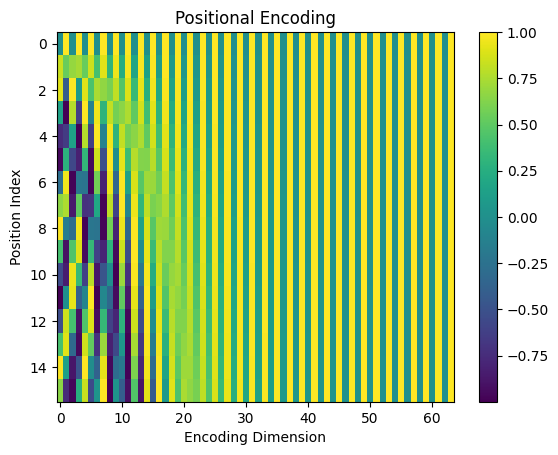
Each vertical line is our dimension from 0 to 64; each row represents a character. The values are between -1 and 1 since they are from sine and cosine functions. Darker colors indicate values closer to -1, and brighter colors are closer to 1. Green colors indicate values in between.
Let's go back to our positional encoding matrix, as you can see, this positional encoding table has the same shape as each batch in the input embedding table [4, 16, 64], they are both (context_length, d_model) = [16, 64].
Since two matrices with same shape can be summed together, we then can add the positional information to each of the input embedding rows to get the Final Input Embedding matrix.
the final input embeddings to be fed to the Transformer decoder blocks for training.
This final result matrix is called Position-wise Input Embedding which in a shape of (batch_size, context_length, d_model) = [4, 16, 64].
This is all about Positional Encoding.
But why use sine and cosine function to encode position? Why not just a random number? Why does summing the two numbers can contain both its meaning and position information? Well, I had the exact same wonderment at the beginning. However, I discovered that it isn't necessary to fully comprehend its underlying mathematics in order to train a model. Therefore, if you are eager for detailed explanations, please refer to the separate section or watch my video clips. I will leave it at that and proceed to the next step.
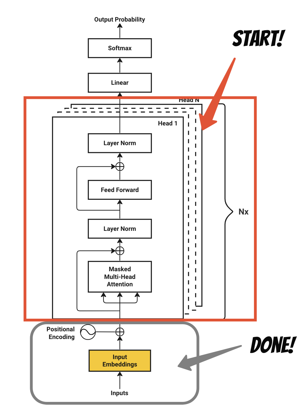
So far we've been covered the input encoding and positional encoding parts of the model. Let's move to the Transformer Block.
Step 4 : Transformer Block
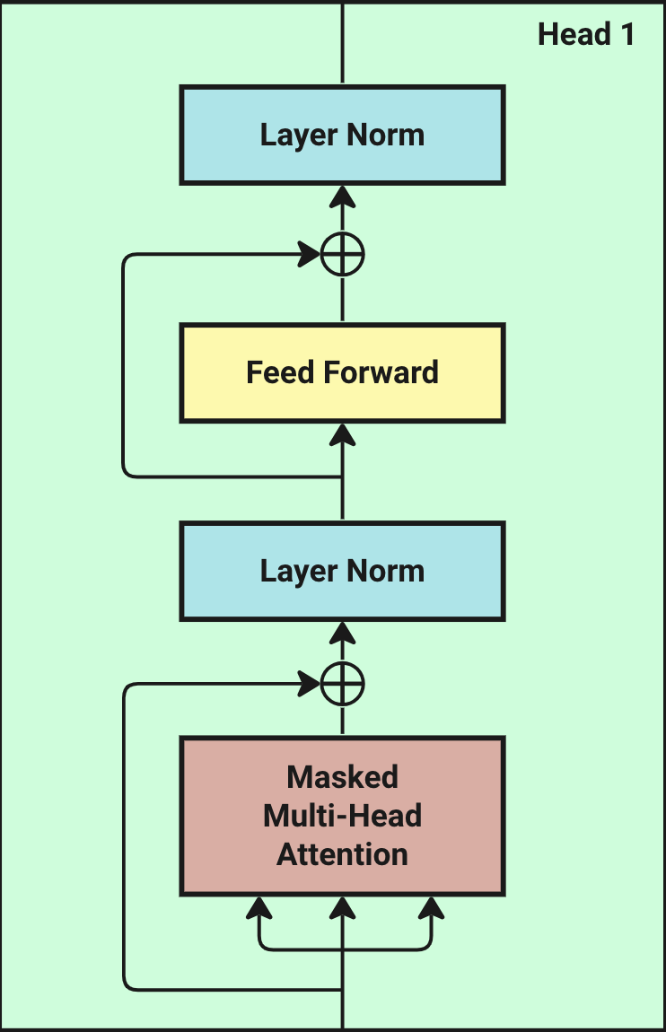
A Transformer block is a stack of three layers: a masked multi-head attention mechanism, two normalization layers and a feed-forward network.
The masked multi-head attention is a set of self-attentions, each of which is called a head. So let's first look at the self-attention mechanism.
4.1 Multi-Head Attention Overview
Transformers get their strength from something called self-attention. With self-attention, the model pays close attention to the most critical parts of the input. Each part is called a head.
This is how a head works: A head works by processing the input through three unique layers called queries (Q), keys (K), and values (V). It starts by comparing Q and K, adjusting the results, and then using these comparisons to create a set of scores showing what's important. These scores are then used to weigh the information in V, giving more attention to the important parts. The head's learning comes from adjusting the settings in these Q, K, and V layers over time.
Multi-head attention simply consists of several individual heads stacked together. All heads receive the exact same input, although they employ their own specific sets of weights during computation. After processing the input, the outputs from all the heads are concatenated and then passed through a linear layer.
Following figure provides a visual representation of the processes within a head, and details in Multi-head Attention block.
In order to perform the attetion calculation, let's bring the formula from original paper "Attention is all you need":

From the formula, we first require three matrices: Q (queries), K (keys), and V (values). To compute the attention scores, we need to perform the following steps:
multiply Q by K transpose (denoted as K^T)
divide by the square root of dimension of K
apply softmax function
multiply by V
We'll go through one by one.
4.2 Prepare Q,K,V
The first step to calculating attention is to acquire the Q, K, and V matrices, representing query, key, and value. These three values will be used in our attention layer to calculate the attention probabilities(weights). These are determined by applying our Position-wise Input Embedding matrix from previous step, denoted as X, to three distinct linear layers labeled Wq, Wk, and Wv (all values are randomly assigned first and learnable). The output of each linear layer is then split into a number of heads, denoted as num_heads, here we choose 4 heads.
The Wq, Wk, Wv are three matrices defined with dimension of (d_model, d_model) = [64, 64]. All values are randomly assigned. This in neural network is called a linear layer or trainable parameters. The trainable parameters are the values that the model will learn and self-update during training.
To obtain our Q,K,V values, we do matrix multiplication between our input embedding matrix X and each of the three matrices Wq, Wk, Wv (once again, their initial values are randomly assigned).
Q = X*Wq
K = X*Wk
V = X*Wv
The calculation(matrix multiplication) logic of the above function:
X is in shape of (batch_size, context_length, d_model) = [4, 16, 64], we break it into 4 sub-matrices of shape [16, 64]. While Wq, Wk, Wv are in shape of (d_model, d_model) = [64, 64]. We can do matrix multiplication on each of the 4 X's sub-matrix against Wq, Wk, Wv.
If you recall linear algebra, the multiplication of two matrices is only possible when the number of columns in the first matrix is equal to the number of rows in the second matrix. In our case, the number of columns in X are 64, and the number of rows in Wq, Wk, Wv are also 64. Therefore, the multiplication is possible.
The matrix multiplication result in shape of 4 sub-matrices of shape [16, 64], which can be combined expressed as (batch_size, context_length, d_model) = [4, 16, 64].
Now, we have our Q, K, V matrices in shape of (batch_size, context_length, d_model) = [4, 16, 64]. Next we need to split them into multiple heads. This is why the transformer architecture name it as Multi-Head Attention.
Splitting heads simply means out of the 64 dimensions of our d_model, we cut them into multiple heads, each head contains a certain number of dimensions. Each head will be able to learn certain patterns or semantics of the input.
Let's say we set our num_heads to be 4 as well. This means we will split our Q, K, V matrices of shape [4, 16, 64] into multiple sub-matrices.
The actual splitting is done by reshaping the last dimension of 64 into 4 sub-dimensions of 16.
Each Q, K, V matrices transformed from shape [4, 16, 64] to [4, 16, 4, 16]. The last two dimensions are the heads. In other words, it transformed from:
[batch_size, context_length, d_model]
to:
[batch_size, context_length, num_heads, head_size]
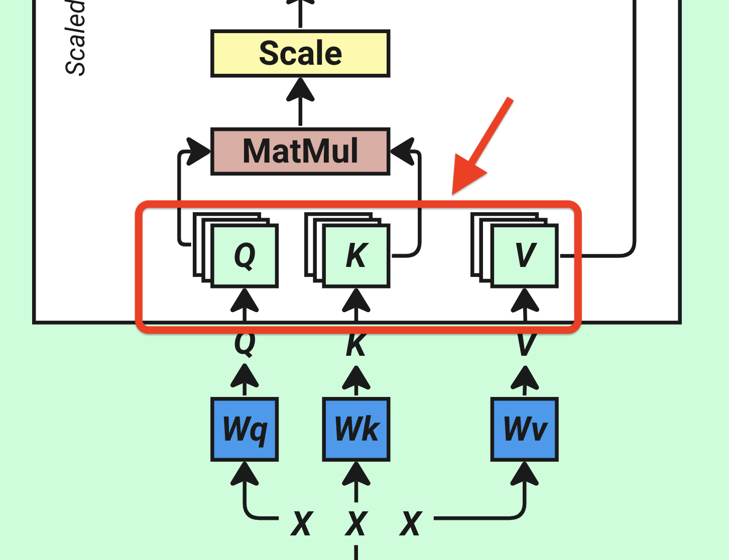
To understand the Q, K, and V matrices with identical shapes [4, 16, 4, 16], consider the following perspective:
In the pipeline, there are four batches. Each batch consists of 16 tokens (words). For every token, there are 4 heads, and each head encodes 16 dimensions of semantic information.
4.3 Calculate Q,K Attention

Now that we have all three matrices of Q, K and V, let’s start calculating single-head attention step by step.
From the diagram of transformer, the Q and K matrices are multiplied first.
Now, if we discard the batch_size from the Q and K matrices with retaining only the last three dimensions, now Q = K = V = [context_length, num_heads, head_size] = [16, 4, 16].
We need to do another transpose on the first two dimensions, to make them in shape of Q = K = V = [num_heads, context_length, head_size] = [4 ,16, 16]. This is because we need to do matrix multiplication on the last two dimensions.
Q * K^T = [4, 16, 16] * [4, 16, 16] = [4, 16, 16]
Why do we do this? The transposition here is done to facilitate matrix multiplication between different contexts. It's more straightforward to explain with a diagram. The last two dimensions, represented as [16, 16], can be visualized as follows:
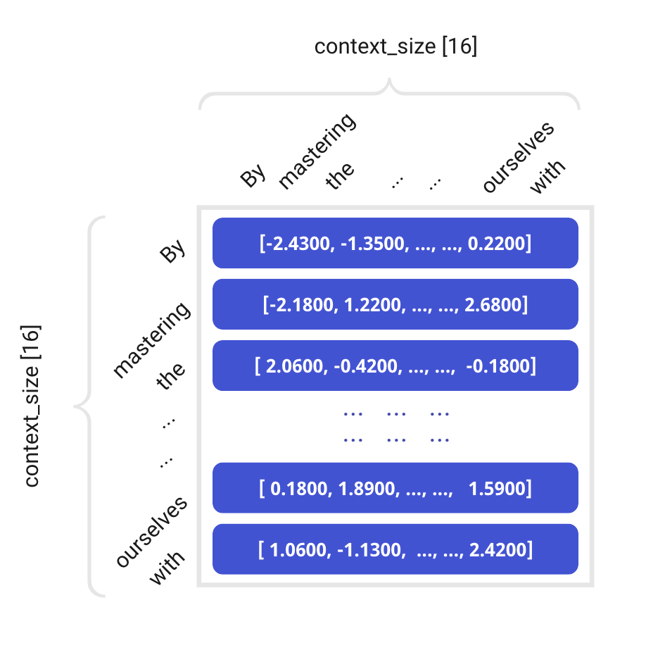
This matrix, where each row and each column represents a token(word) in the context of our example sentence. The matrix multiplication is the measurement of similarity between each word and every other word in the context. The higher the value, the more similar they are.
Let me bring up one head of the attention score:
The numbers in this 16 by 16 matrix represent attention scores of our example sentence " . By mastering the art of identifying underlying motivations and desires, we equip ourselves with ".
It is easier to see as a plot:
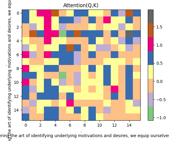
The horizontal axis represents one of Q's head, the vertical axis represents one of K's head, colored squares represent the similarity score between each token and each other token in the context. The darker the color, the higher the similarity.
The similarities shown above of course don't make much sense now, because those are just from randomly assigned values. But after training, the similarity scores will be meaningful.
OK, now let's bring the batch dimension, batch_size, back into the Q*K attention scores. The final result will have the shape [batch_size, num_heads, context_length, head_size], which is [4, 4, 16, 16].
This is the Q*K Attention Score at current step.
4.4 Scale

The scale part is quite straightforward, we just need to divide the Q*K^T attention score by the square root of the dimension of K.
Here, our dimension of K equals to the dimension of Q, which is d_model divided by num_heads: 64/4 = 16.
Then we take the square root of 16, which is 4. And divide the Q*K^T attention score by 4.
The reason of doing this is to prevent the Q*K^T attention score from being too large, which could cause the softmax function to saturate, which in turn could cause the gradient to vanish.
4.5 Mask
In the decoder-only transformer model, masked self-attention essentially functions as sequence padding.
Decoder could only view the previous characters, but not the future characters. So the future characters are masked out and used for calculating the attention weights.
This is very easy to understand if we visualize the plot again:
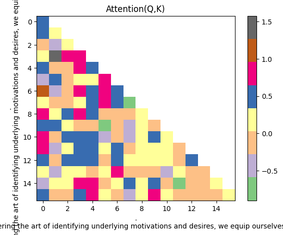
white spaces means scores in 0, which are masked out
The point of masking in the multi-headed attention layer is to prevent the decoder from “seeing into the future”. In our example sentence, the decoder is only allowed to see the current word and all the words that came before it.
4.6 Softmax

The softmax step changes numbers into a special kind of list, where the whole list adds up to one. It increases high numbers and decreases low ones, creating clear choices.
In a nutshell, the softmax function is used to convert the output of the linear layer into a probability distribution.
In modern deep learning frameworks, like PyTorch, the softmax function is a built-in function which quite straightforward to use:
This line of code will apply the softmax to all attentions scores we calculated in previous step and result in a probability distributions between 0 and 1.
Let's also bring up the same head's attention scores after applying softmax:
all the probability scores are now positive and add up to 1.
4.7 Calculate V Attention

The last step is to multiply the softmax output with the V matrix.
Remember, our V matrix also split it into multiple heads in shape of (batch_size, num_heads, context_length, head_size) = [4, 4, 16, 16].
While the output from previous softmax step is in shape of (batch_size, num_heads, context_length, head_size) = [4, 4, 16, 16].
Here we perform another matrix multiplication on the last two dimensions of both matrices.
softmax_output * V = [4, 4, 16, 16] * [4, 4, 16, 16] = [4, 4, 16, 16]
The result is in shape of [batch_size, num_heads, context_length, head_size] = [4, 4, 16, 16].
We call this result A.
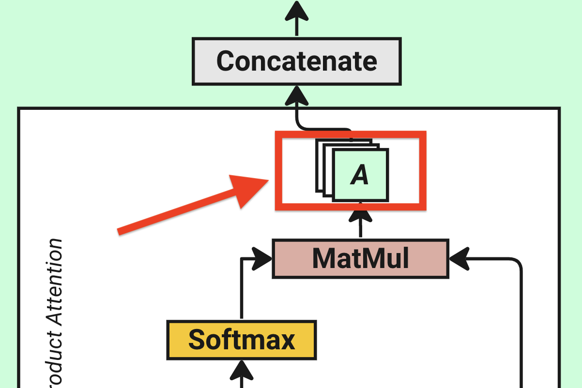
4.8 Concatenate and Output
The final step of our multi-head attention is to concatenate all the heads together and pass them through a linear layer.
The ideal of concatenation is to combine the information from all heads together. Thus, we need to reshape our A matrix from [batch_size, num_heads, context_length, head_size] = [4, 4, 16, 16] to [batch_size, context_length, num_heads, head_size] = [4, 16, 4, 16]. The reason is that we need to put num_heads and head_size back together to the last two dimensions, so will easily combine them (by doing matrix multiplication) back to size d_model = 64.
This can be easily done through PyTorch's built-in function:
Next, we need to combine the last two dimensions [num_heads, head_size] = [4, 16] to [d_model] = [64].
As you can see, after series of calculations our result matrix A is now back to the shape same as our input embedding matrix X, which is [batch_size, context_length, d_model] = [4, 16, 64]. Since this output result will be passed to the next layer as the input, so keeping the input and output the same shape is necessary.
But before passing it to the next layer, we need perform another linear transformation on it. This is done by doing another matrix multiplication between the concatenated matrix A and Wo.
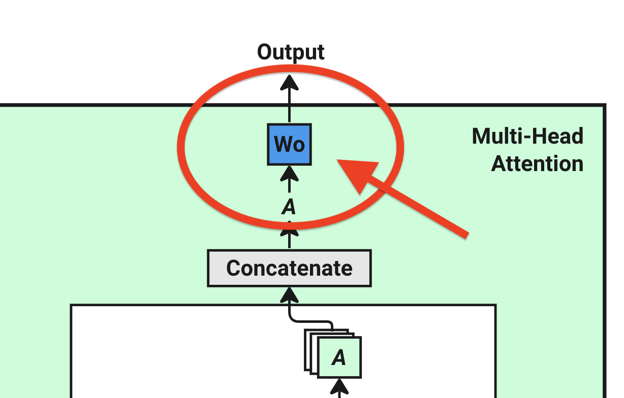
This Wo is randomly assigned with shape [d_model, d_model] and will be updated during training.
Output = A* Wo = [4, 16, 64] * [64, 64] = [4, 16, 64]
The output of the linear layer is the output of the single-head attention, denoted as output.
Congratulations! Now we have finished the masked multi-head attention part! And let's start the rest of the transformer block. Those are quite straightforward, so I will go through them quickly.
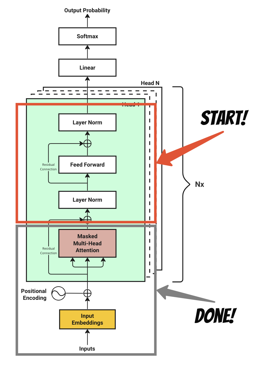
Step 5 : Residual Connection and Layer Normalization
A residual connection, sometimes referred as a skip connection, is a connection that let original input X bypasses one or more layers.
This is simply a summation of the original input X and the output of the multi-head attention layer. Since they are in same shape, adding them up is straightforward.
After the residual connection, the process goes to layer normalization. LayerNorm is a technique that normalizes the outputs of each layer in the network. This is done by subtracting the mean and dividing by the standard deviation of the layer's outputs. This technique is used to prevent the outputs of a layer from becoming too large or too small, which can cause the network to become unstable.
This is also single line of code in PyTorch using nn.LayerNorm function. We will see in action in the Let's Code LLM section.
The residual connection and layer normalization are denoted as Add & Norm in the diagram of "Attention is All You Need"'s original paper.
Step 6 : Feed-Forward Network
Once we have the normalized attention weights (probability scores), it will be processed through a position-wise feedforward network.
The feed-forward network (FFN) consists of two linear layers with a ReLU activation function between them. Let's see how the python code implements this:
Take the ChatGPT explanation to the above code:
output = nn.Linear(d_model, d_model * 4)(output): This applies a linear transformation to the incoming data, i.e., y = xA^T + b. The input and output sizes are d_model and d_model * 4, respectively. This transformation increases the dimensionality of the input data.
output = nn.ReLU()(output): This applies the Rectified Linear Unit (ReLU) function element-wise. It's used as an activation function that introduces non-linearity to the model, allowing it to learn more complex patterns.
output = nn.Linear(d_model * 4, d_model)(output): This applies another linear transformation, reducing the dimensionality back to d_model. This kind of "expansion then contraction" is a common pattern in neural networks.
As someone new to machine learning or LLM, like you and me, could have get lost by these explanations. I got exactly same feeling when I first encounter these terms.
But no worries, we can understand it like this: this feed-forward network is just a standard neural network module whose input and output are both attention scores. Its purpose is to expand the dimensionality of the attention scores from 64 to 256, which makes the information more granular and enables the model to learn more complex knowledge structures. Then, it compresses the dimensions back down to 64, making it suitable for subsequent computations.
Step 7 : Repeat Step 4 to 6
Cool! We have finished the first transformer block. Now we need to repeat the same process for the rest of the number of transformer blocks we want to have.
In terms of heads, I quoted from HuggingChat's AI response:
By having multiple blocks, the output is trained and being passed into next block as input X, so after iterations the model can learn more complex patterns and relationships between the words in the input sequence.
Step 8 : Output Probabilities
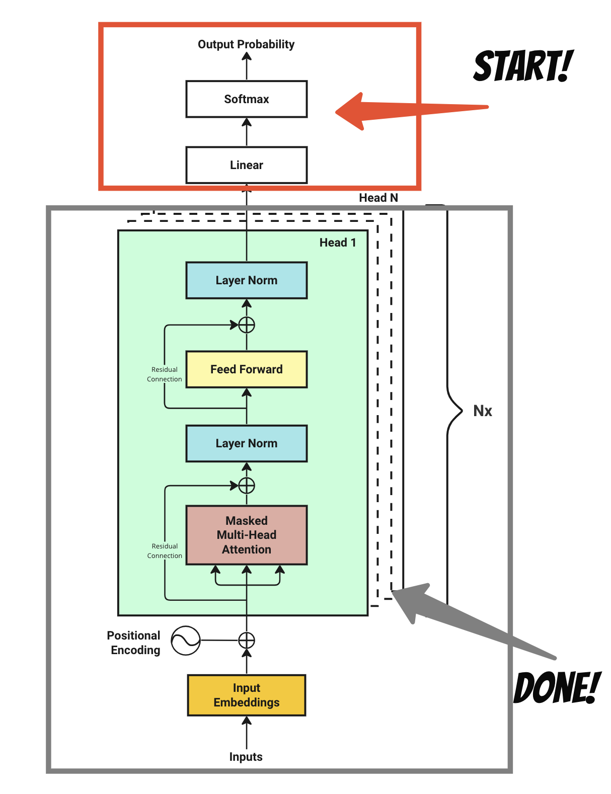
During inference, you want to get the next predicted token from the model, but what we get so far is actually a probability distribution of all the tokens in the vocabulary. Do you still recall our vocabulary size is 3,771 in the example above? So in order to select one of the highest probability token, we will form a matrix with the size of the model dimensions d_model = 64 by our vocab_size = 3,771. This step is no difference in training than in inference.
We call the output after this linear layer the logits. The logits is a matrix of shape [batch_size, context_length, vocab_size] = [4, 16, 3771].
Then a final softmax function is used to convert the logits of the linear layer into a probability distribution.
Note: during training, we don't need to apply softmax function here, but instead use nn.CrossEntropy function since it build-in softmax behaviours.
How do we look into the resulting logits of shape [4, 16, 3771]? Actually after all the calculations it's quite a simple idea:
We have 4 batch pipelines, each pipeline contains all the 16 words in that input sequence, with each word mapped to a probability against every other word in the vocabulary.
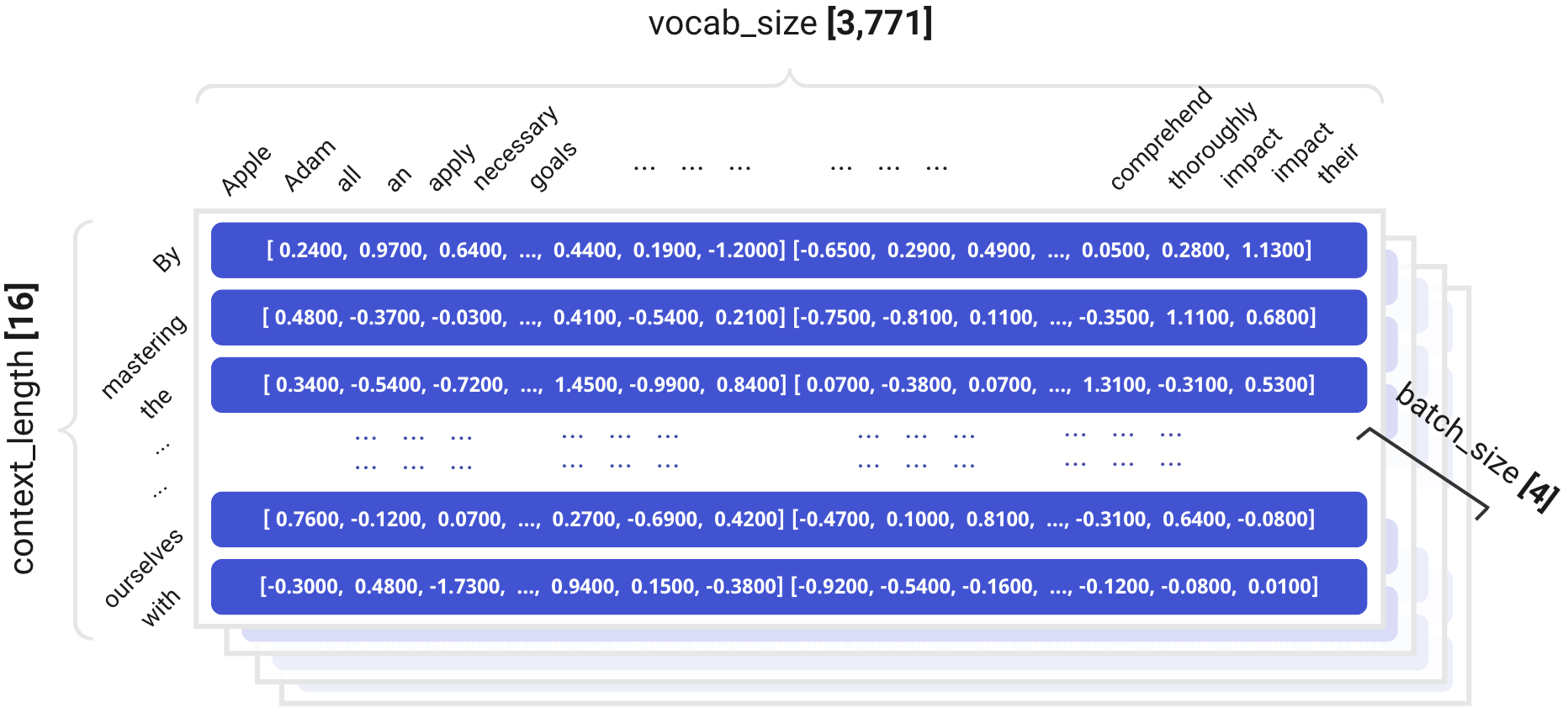
If the model is in training, we update those probability parameters, if the model is in inference, we simply select one with the highest probability. Then everything makes sense.
Conclusion
Typically, it can be challenging to grasp the complexities of the Transformer architecture entirely during the initial exposure. Personally, it required approximately a month for me to thoroughly comprehend every component within the system. Therefore, I would suggest reviewing additional resources listed on our reference page and gaining inspiration from other remarkable Trailblazers.
On a personal note, I find videos more effective as tutorials. To facilitate learning, I have prepared several video explanations covering concepts and hands-on coding experience related to this architecture. They shall be available shortly.
Once you feel confident about understanding the Transformer architecture, moving forward to implementing the code through a series of guided steps would be advisable. Exciting progress awaits!